Traditionally, machine learning (ML) (opens new window) can be classified broadly into two types: supervised and unsupervised learning (opens new window). In supervised learning, we have some data with labels and these labels are used to train the model. For example, using the (labelled) images of different objects to train an image classifier.
Unsupervised learning, on the other hand, doesn’t require any labelling and here we explore the patterns without any prior information. Inevitably, it's difficult but appealing too. With tons of data available (and new data produced every day), it's always easy to get the data, though getting it labelled requires a lot of time and money.
To harness the heaps of data available around us, there is an advanced learning strategy, known as self-supervised learning. In self-supervised learning, we take the unlabelled data and mimic supervised learning.
# Self-Supervised Learning (SSL)
In self-supervised learning, we partition the data into positive and negative samples - similar to binary (supervised) classification - by treating the object under consideration as a positive example and all the other samples as negative.
Self-supervised learning methods learn joint embeddings and can be broadly classified into two types:
- Contrastive methods
- Non-contrastive methods
In contrastive methods, we take different samples of the same data, like different views of the same image and try to maximize their similarity scores, while trying to minimise them for the other samples/images. Non-contrastive methods, on the other hand, don’t account for the negative samples. Some of the famous SSL methods like BYOL or DINO are good examples of non-contrastive methods, while SimCLR and MoCo use negative examples too and are good examples of contrastive methods.
# Contrastive Learning (CL)
Contrastive learning centres around a simple concept of choosing a representation that maximizes the similarities between positive data pairs, while minimizing for negative pairs. For example, I input an image of a mango and now its goal should be to maximize the similarity between mango images while minimizing it for some other images.
The simplest setting is to consider each data point (when considering it) as a positive data point while considering everyone else as a negative point. Let’s suppose the point is
# Training
For each pair of data points
To make the training more practical, we perform it in batches and let's say we have a batch of 32 images, then 1 image (itself) needs to have a maximized similarity score, while the other 31 will have to have as much minimized similarity score as possible.
However, having a single positive vs a number of negative examples makes it quite hard to learn discriminative features, so we employ some smart techniques like data augmentation to make multiple copies of the same data point.
# CL Examples
Contrastive Learning has been there for some time. In the last 10 years, it has come a long way from normal CNN-based (opens new window) image discrimination (which was just happy to outperform SIFT) to CLIP. Some of the modern CL algorithms are:
- Contrastive Predictive Coding, CPC
- A simple framework for Contrastive Learning of (visual) Representations, SimCLR
- Momentum Contrast, MoCo
- Contrastive Language-Image Pretraining, CLIP
Let’s go through them briefly to get a better idea of how contrastive learning is being used practically.
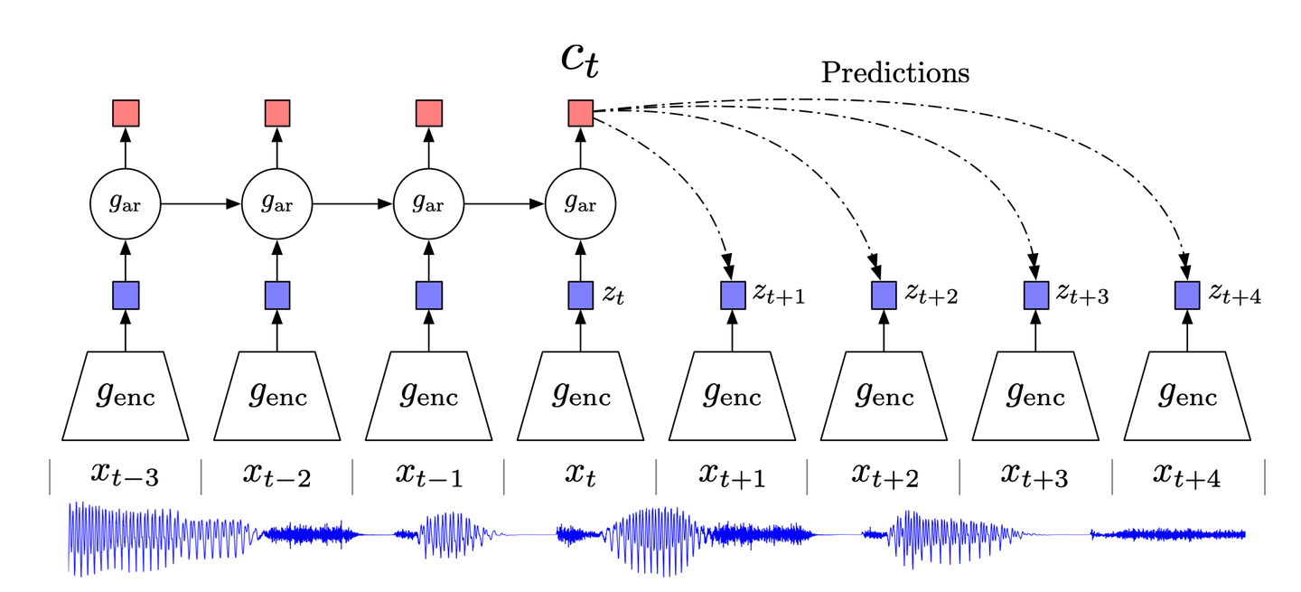
# Contrastive Predictive Coding
Inspired by the classical data compression technique of predictive coding and its adaptation in neuroscience, CPC (Contrastive Predictive Coding) (opens new window) tries to focus on the high-level information in the data, while ignoring the low-level/noise.
CPC, in a nutshell, works as follows:
- High-dimensional data is compressed into a suitable latent embedding space. This compression makes it easier to model the data and make predictions accordingly.
- Predictions are made in the chosen embedding space.
- The model is trained using the Noise-Contrastive Estimation (NCE) loss function.
# SimCLR
A Simple framework for Contrastive Learning of visual Representations, SimCLR is an advanced contrastive learning technique for computer vision. Without needing any pre-augmentation or specialized architecture, SimCLR works as follows:
- An image is chosen randomly and its views (two in the original implementation) are generated using different augmentation techniques like random cropping, random colour distortion or Gaussian blurring.
- Image representation/embedding is computed using a ResNet-based CNN.
- This representation is further transformed into a (non-linear) projection using an MLP.
- Both CNN and MLP are trained to minimize the contrastive loss function.
Throughout, we have been talking about the need for unsupervised learning, but we have some labelled data at our disposal too. In the end, if we fine-tune the CNN on some labelled images, it helps increase its performance and generalization on diverse other (downstream) tasks.
Some insights on how Contrastive Learning works
Not only did SimCLR introduce a new model with very good performance (you can check its paper for a detailed results analysis), but its authors also gave some new insights which can be useful for almost any contrastive learning method. So I found them worthy of sharing here:
A combination of augmentation techniques is critical: Random cropping and colour distortion didn’t give standout results when used individually, but when used in conjunction, they give the best results.
Nonlinear projection is important: The complex nature of neural networks and contrastive loss function means it's hard to understand what’s going on behind the scenes, but empirically it is clear that the non-linear projection (by MLP) is useful as it increases the performance up to 10%. This fact will be independently observed in the MoCov2’s publication too, as we will shortly see.
Scaling up improves performance: While some of the observations are specific to SimCLR, they are mainly generic across contrastive learning. Increasing the model’s capacity (either width or depth), increasing the batch size or even the number of epochs all lead to an increase in performance.
# Momentum Contrast (MoCo)
Momentum Contrast (MoCo) takes an alternative view of contrastive learning as a dictionary lookup. This interesting point of view, having some similarities with the transformer models, works as follows:
- Data augmentation is applied to produce two copies,
- Query encoder (one on the left in the image below) takes the
- The momentum encoder takes the other augmented copy, xk and dynamically generates a dictionary of keys,
To make it relevant, it is implemented as a queue, which takes
- Encoded query,
- Both encoders are trained together to minimize this contrastive loss.
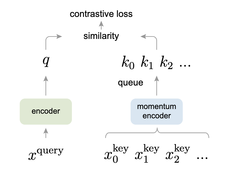
If you are familiar with transformers, you can see that InfoNCE loss is quite similar to the way we calculate attention in the transformers.
# CLIP
Introduced in 2021, CLIP ups the ante by combining both images and their captions. While it doesn’t work in a momentum-based averaging way, it also works with two encoders, one for text and the other one for images. Here’s its brief workflow:
- The Image is entered into the image encoder and its caption is entered in the text encoder.
- Image encoder, based on a ViT (Vision Transformer) gets the image embedding, while text encoder tokenizes the caption to get the text features. These features are collated as a pair in the embedding space.
- Both text and image encoders are trained in a way to maximize the distance of any given pair of
- While testing, we provide a dictionary of captions (not to be confused with the dynamic dictionary in MoCo) and the desired image. Based on the image, it returns the caption having the highest probability.
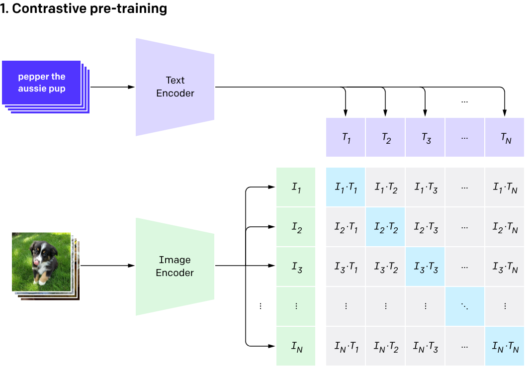
Note: For more details about CLIP, please read this (opens new window).
# Code Example
Let's wrap things up with a code example to complete the picture. Here, I will be using the official implementation of MoCo (opens new window) by Meta Research. This code mainly centres around the Moco class.
# Constructor
MoCo class’s constructor initializes the attributes like K, m and T. As we can see, it uses the default values of feature dimension (dim) as 128, queue size (K) as 16-bits (65,536), while momentum co-efficient,μ is 0.999 (quite slow moving average). Softmax temperature τ, as already specified in the paper is 0.07.
Also, we can see the implementation of MLP which we saw first in the SimCLR, and later on in the MoCov2 (this implementation includes both versions).
def __init__(self, base_encoder, dim=128, K=65536, m=0.999, T=0.07, mlp=False):

        super(MoCo, self).__init__()

        self.K = K
        self.m = m
        self.T = T

        # create the encoders
        # num_classes is the output fc dimension
        self.encoder_q = base_encoder(num_classes=dim)
        self.encoder_k = base_encoder(num_classes=dim)

        if mlp:  # hack: brute-force replacement
            dim_mlp = self.encoder_q.fc.weight.shape[1]
            self.encoder_q.fc = nn.Sequential(
                nn.Linear(dim_mlp, dim_mlp), nn.ReLU(), self.encoder_q.fc
            )
            self.encoder_k.fc = nn.Sequential(
                nn.Linear(dim_mlp, dim_mlp), nn.ReLU(), self.encoder_k.fc
            )

        for param_q, param_k in zip(
            self.encoder_q.parameters(), self.encoder_k.parameters()
        ):
            param_k.data.copy_(param_q.data)  # initialize
            param_k.requires_grad = False  # not update by gradient

        # create the queue
        self.register_buffer("queue", torch.randn(dim, K))
        self.queue = nn.functional.normalize(self.queue, dim=0)

        self.register_buffer("queue_ptr", torch.zeros(1, dtype=torch.long))
# Momentum Encoder
The core part is simple yet so effective. In the momentum encoder, we are simply implementing this equation for momentum-based average:
@torch.no_grad()
    def _momentum_update_key_encoder(self):

        for param_q, param_k in zip(
            self.encoder_q.parameters(), self.encoder_k.parameters()
        ):
            param_k.data = param_k.data * self.m + param_q.data * (1.0 - self.m)
# Queue Management
Finally, the queue is updated to remove the older batch data. It works as follows:
- We gather the keys first
- Queue’s pointer points to the
keystranspose. Now, why it is done precisely for the columns and not rows is something I am curious about. - In the end, the pointer moves to the next batch (modulus here is for the circular queue) and it’s reflected in the attribute (
self.queue_ptr) too.
 def _dequeue_and_enqueue(self, keys):

        keys = concat_all_gather(keys)
        batch_size = keys.shape[0]
        ptr = int(self.queue_ptr)
        assert self.K % batch_size == 0

        self.queue[:, ptr : ptr + batch_size] = keys.T
        ptr = (ptr + batch_size) % self.K
        self.queue_ptr[0] = ptr
# Training
In the training pass, we combine this all as:
- Computing query features
- Computing key features (using the momentum update)
- Computing the logits (both positive and negative)
- Dequeue and enqueue using the function we just discussed above
def forward(self, im_q, im_k):
        """
        Input:
            im_q: a batch of query images
            im_k: a batch of key images
        Output:
            logits, targets
        """

        # compute query features
        q = self.encoder_q(im_q)  # queries: NxC
        q = nn.functional.normalize(q, dim=1)

        # compute key features
        with torch.no_grad():  # no gradient to keys
            self._momentum_update_key_encoder()  # update the key encoder

            # shuffle for making use of BN
            im_k, idx_unshuffle = self._batch_shuffle_ddp(im_k)

            k = self.encoder_k(im_k)  # keys: NxC
            k = nn.functional.normalize(k, dim=1)

            # undo shuffle
            k = self._batch_unshuffle_ddp(k, idx_unshuffle)

        # compute logits
        # Einstein sum is more intuitive
        # positive logits: Nx1
        l_pos = torch.einsum("nc,nc->n", [q, k]).unsqueeze(-1)
        # negative logits: NxK
        l_neg = torch.einsum("nc,ck->nk", [q, self.queue.clone().detach()])

        # logits: Nx(1+K)
        logits = torch.cat([l_pos, l_neg], dim=1)

        # apply temperature
        logits /= self.T

        # labels: positive key indicators
        labels = torch.zeros(logits.shape[0], dtype=torch.long).cuda()

        # dequeue and enqueue
        self._dequeue_and_enqueue(k)

        return logits, labels
By the way, all these comments are written by the authors themselves and show that not only did they write a clear paper, but written a good, easy-to-understand code too.

# Contrastive Learning and Vector Databases
Since contrastive learning centres around the input data embeddings and their distance, they are highly relevant to vector databases. Using a trained CL model, we can simply apply a metric like Euclidean distance, Cosine similarity or
As a result, we can have countless applications of contrastive learning in conjunction with vector databases, for example:
- Zero-shot recognition (can have a number of applications itself) using CLIP
- Recommendation system for an online user - based on the user’s history, it will suggest the products having the closest proximity to those embeddings.
- Document retrieval - retrieve the document from the database which is closest to the user’s query embedding
- Anomaly detection - whether a new transaction by this credit card is normal or fraudulent can be checked using the previous transaction embeddings and finding the similarity (or dissimilarity) between this transaction and the transaction history’s “region” in the embedding space.
# References
- Dosovitskiy, et al., Discriminative Unsupervised Feature Learning with Exemplar Convolutional Neural Networks, IEEE PAMI, 2016.
- Hjelm, et al., Learning Deep Representations by Mutual Information Estimation and Maximization, ICLR, 2019.
- Oord, et al., Representation Learning with Contrastive Predictive Coding, arXiv 2018.
- Chen, et al., A Simple Framework for Contrastive Learning of Visual Representations, ICML 2020.
- Radford, et al., Learning Transferable Visual Models From Natural Language Supervision, arXiv 2020
- He, et al., Momentum Contrast for Unsupervised Visual Representation Learning, arXiv 2020
- He, et al., Improved Baselines with Momentum Contrastive Learning, arXiv 2020