In our ongoing exploration of advanced RAG, we've covered the core principles and applications of this powerful technique. Now, we turn our attention to a crucial component that underpins the efficiency of the RAG process: vector indexing. By the way, you can also find other blogs of this series here:
Topics:
Indexing Methods in Advanced RAG
Indexing has long been a vital tool in database management, enabling rapid retrieval of information. Much like how a library catalog helps you quickly locate a specific book, indexing in databases allows for streamlined access to data. In the context of RAG, vector indexing takes this concept to new heights, facilitating the efficient retrieval of relevant information from knowledge bases.
In this installment of the Advanced RAG blog series, we will delve into the fundamentals of vector indexing and explore how it is implemented using various techniques. By understanding the power of vector indexing, you'll be equipped to unlock the full potential of your RAG-powered applications, delivering more informed and contextual outputs. Let's dive in and discover how vector indexing can elevate your Retrieval Augmented Generation strategies.
# What are Vector Embeddings
Vector embeddings are simply the numerical representation that is converted from images, text, and audio. In simpler terms, a single mathematical vector is created against each item capturing the semantics or characteristics of that item. These vector embeddings are more easily understood by computational systems and compatible with machine learning models to understand relationships and similarities between different items.
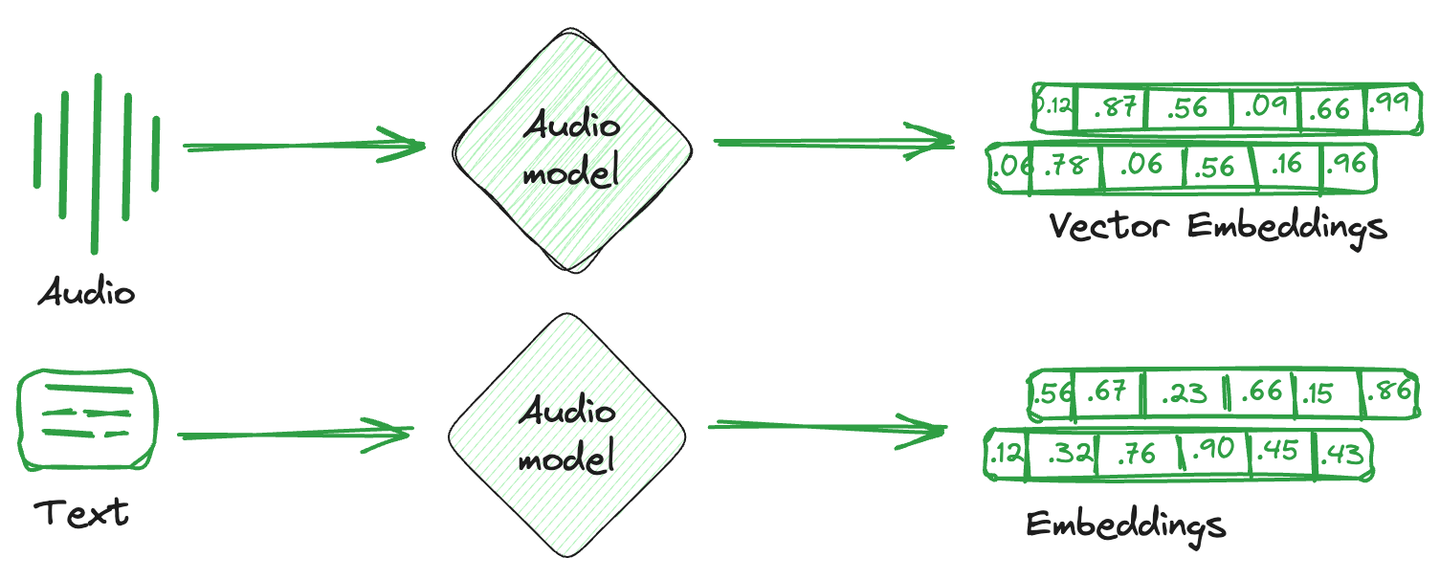
Specialized databases used to store these embedding vectors are known as vector databases. These databases take advantage of the mathematical properties of embeddings that allow similar items to be stored together. Different techniques are used to store similar vectors together and dissimilar vectors apart. They are vector indexing techniques.
# What is a Vector Index
Vector indexing is not just about storing data, it’s about intelligently organizing the vector embeddings to optimize the retrieval process. This technique involves advanced algorithms to neatly arrange the high-dimensional vectors in a searchable and efficient manner. This arrangement is not random; it’s done in a way that similar vectors are grouped together, by which vector indexing allows quick and accurate similarity searches and pattern identification, especially for searching large and complex datasets.
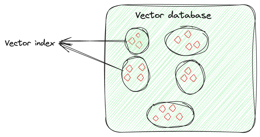
Let's say you have a vector for each image, capturing its features. The vector index will organize these vectors in a way that makes it easier to find similar images (here). You can think of it as if you are organizing each person's images separately. So, if you need a specific person's picture from a particular event, instead of searching through all the pictures, you would only go through that person's collection and easily find the image.
# Common Vector Indexing Techniques
Different indexing techniques are used based on specific requirements. Let’s discuss some of these.
# Inverted File (IVF)
This is the most basic indexing technique. It splits the whole data into several clusters using techniques like K-means clustering. Each vector of the database is assigned to a specific cluster. This structured arrangement of vectors allows the user to make the search queries way faster. When a new query comes, the system doesn't traverse the whole dataset. Instead, it identifies the nearest or most similar clusters and searches for the specific document within those clusters.
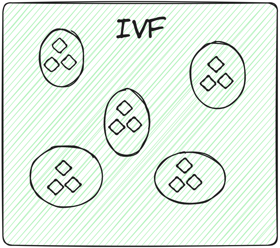
So, applying brute-force search exclusively within the relevant cluster, rather than across the entire database, not only enhances search speed but also considerably reduces query time.
# Variants of IVF: IVFFLAT, IVFPQ and IVFSQ
There are different variants of IVF, depending on the specific requirement of the application. Let's look at them in detail.
# IVFFLAT
IVFFLAT (opens new window) is a simpler form of IVF. It partitions the dataset into clusters. However, within each cluster, it uses a flat structure (hence the name "FLAT") for storing the vectors. IVFFLAT is designed to optimize the balance between search speed and accuracy.
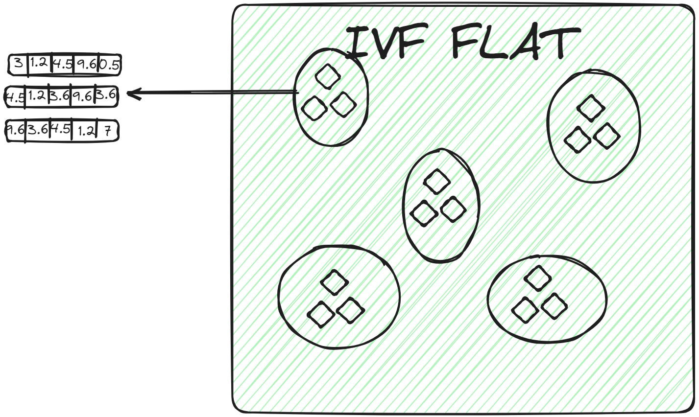
In each cluster, vectors are stored in a simple list or array without additional subdivision or hierarchical structures. When a query vector is assigned to a cluster, the nearest neighbor is found by conducting a brute-force search, examining each vector in the cluster's list and calculating its distance to the query vector. IVFFLAT is employed in scenarios where the dataset isn't considerably large, and the objective is to achieve high accuracy in the search process.
# IVFPQ
IVFPQ (opens new window) is an advanced variant of IVF, which stands for Inverted File with Product Quantization. It also splits the data into clusters but each vector in a cluster is broken down into smaller vectors, and each part is encoded or compressed into a limited number of bits using product quantization.
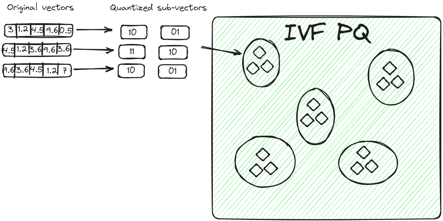
For a query vector, once the relevant cluster is identified, the algorithm compares the quantized representation of the query with the quantized representations of vectors within the cluster. This comparison is faster than comparing raw vectors due to the reduced dimensionality and size achieved through quantization. This method has two advantages over the previous method:
- The vectors are stored in a compact way, taking less space than the raw vectors.
- The query process is even faster because it doesn't compare all raw vectors but encoded vectors.
# IVFSQ
File System with Scalar Quantization (IVFSQ) (opens new window), like other IVF variants, also segments the data into clusters. However, the major difference is its quantization technique. In IVFSQ, each vector in a cluster is passed through scalar quantization. This means that each dimension of the vector is handled separately.
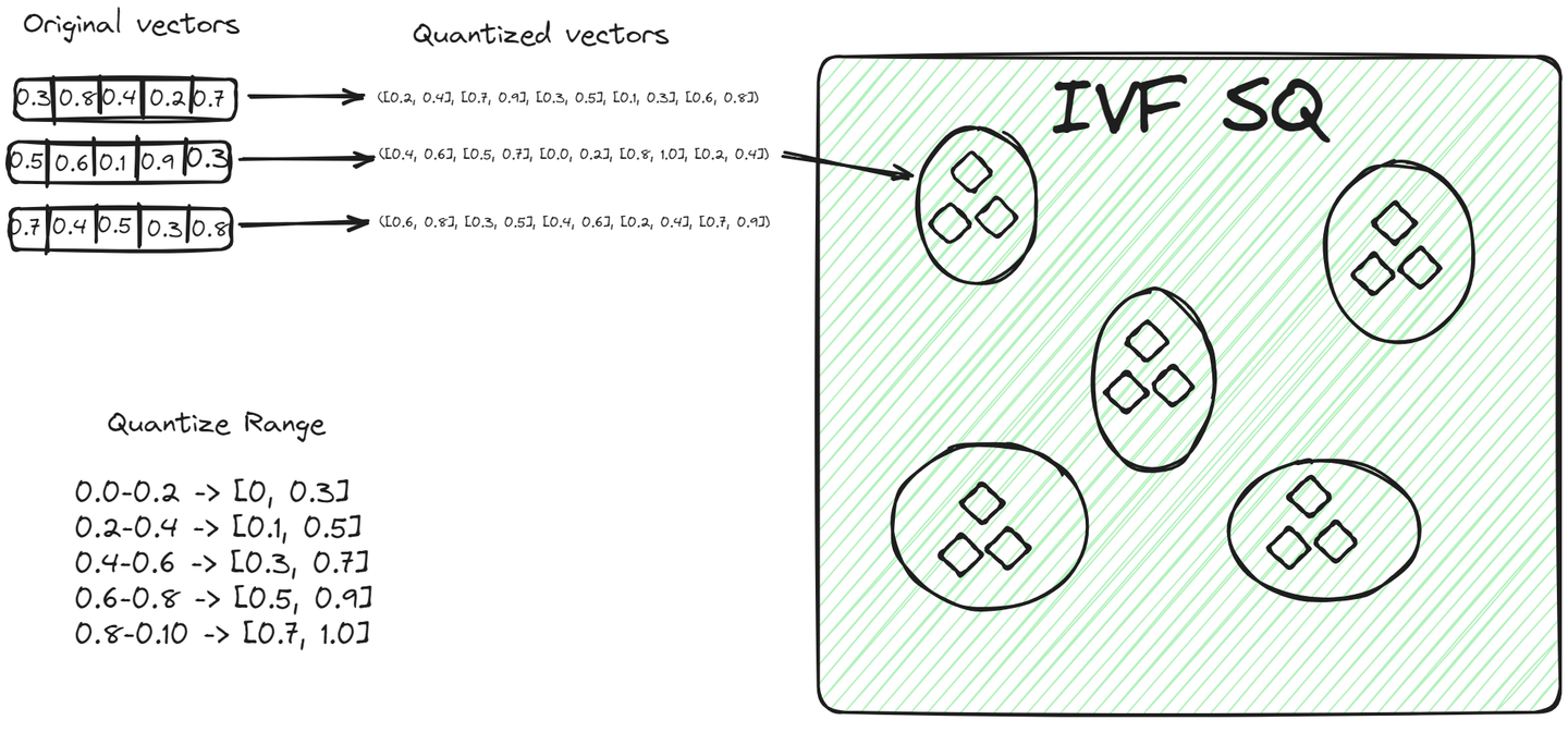
In simple terms, for every dimension of a vector, we set a predefined value or range. These values or ranges help decide which cluster a vector belongs to. Each component of the vector is then matched against these predefined values to find its place in a cluster. This method of breaking down and quantizing each dimension separately makes the process more straightforward. It's especially useful for lower-dimensional data, as it simplifies encoding and reduces the space needed for storage.
# Hierarchical Navigable Small World (HNSW) Algorithm
The Hierarchical Navigable Small World (opens new window) (HNSW) algorithm is a sophisticated method for storing and fetching data efficiently. Its graph-like structure takes inspiration from two different techniques: the probability skip list and Navigable Small World (NSW).
To better understand HNSW, let's first try to understand the basic concepts related to this algorithm.
# Skip List
A skip list is an advanced data structure that combines the advantages of two traditional structures: the quick insertion capability of a linked list and the rapid retrieval characteristic of an array. It achieves this through its multi-layer architecture where the data is organized across multiple layers, with each layer containing a subset of the data points.
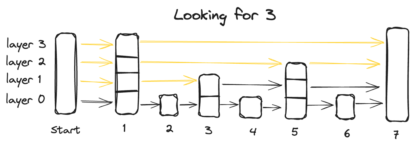
Starting from the bottom layer, which contains all data points, each succeeding layer skips some points and thus has fewer data points, ultimately the topmost layer will have the smallest number of data points.
To search for a data point in a skip list, we start from the highest layer and go from left to right exploring each data point. At any point, if the queried value is greater than the current datapoint, we move back to the previous datapoint in the layer below and resume the search from left to right until we locate the exact point.
# Navigable Small World (NSW)
Navigable Small World (NSW) is similar to a proximate graph where nodes are linked together based on how similar they are to each other. The greedy method is used to search for the nearest neighbor point.
We always begin with a pre-defined entry point, which connects to multiple nearby nodes. We identify which of these nodes are the closest to our query vector and move there. This process iterates until there is no node closer to the query vector than the current one, serving as the stopping condition for the algorithm.
Now, let's get back to the main topic and see how it works.
# How HNSW is Developed
So, what happens in HNSW is that we take the motivation from the skip list, and it creates layers like the skip list. But for the connection between the data points, it makes a graph-like connection between the nodes. The nodes at each layer are connected not only to the current layer nodes but also to the nodes of the lower layers. The nodes at the top are very few and intensity increases when we go down to the lower layers. The last layer contains all the data points of the database. This is what the HNSW architecture looks like.
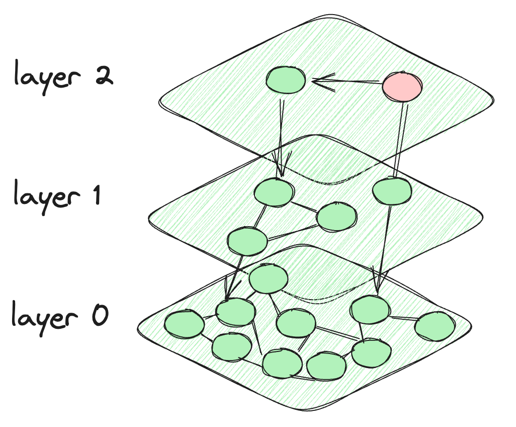
The architecture of the HNSW algorithm
# How Does a Search Query Work in HNSW
The algorithm starts at the predefined node of the topmost layer. It then computes the distance between the connected nodes of the current layer and those in the layer below. The algorithm shifts to a lower layer if the distance to a node in that layer is less than the distance to nodes in the current layer. This process continues until the last layer is reached or it reaches a node that has the minimum distance from all other connecting nodes. The final layer, Layer 0, contains all data points, providing a comprehensive and detailed representation of the dataset. This layer is crucial to ensure that the search incorporates all potential nearest neighbors.
# Different variants of HNSW: HNSWFLAT and HNSWSQ
Just like IVFFLAT and IVFSQ, where one stores raw vectors and the other stores quantized ranges, the same process applies to HNSWFLAT and HNSWSQ. In HNSWFLAT, the raw vectors are stored as they are, while in HNSWSQ, the vectors are stored in a quantized form. Apart from this key difference in data storage, the overall process and methodology of indexing and searching are the same in both HNSWFLAT and HNSWSQ.

# Multi-Scale Tree Graph (MSTG) Algorithm
Standard Inverted File Indexing (IVF) partitions a vector dataset into numerous clusters, while Hierarchical Navigable Small World (HNSW) builds a hirarchical graph for the vector data. However, a notable limitation of these methods is the substantial growth in index size for massive datasets, requiring the storage of all the vector data in memory. While methods like DiskANN can offload vector storage to SSD, it builds index slowly and has very low filtered search performance.
Multi-Scale Tree Graph (MSTG) is developed by MyScale (opens new window) and it overcomes these limitation by combining hierarchical tree clustering with graph traversal, memory with fast NVMe SSDs. MSTG significantly reduces the resource consumption of IVF/HNSW while retaining exceptional performance. It builds fast, searches fast, and remains fast and accurate under different filtered search ratios while being resource and cost-efficient.
# Conclusion
Vector databases have revolutionized the way data is stored, providing not just enhanced speed but also immense utility across diverse domains such as artificial intelligence and big data analytics. In an era of exponential data growth, particularly in unstructured forms, the applications of vector databases are limitless. Customized indexing techniques further amplify the power and effectiveness of these databases, for example, boosting filtered vector search.
With its proprietary MSTG (Multi-Scale Tree Graph) indexing algorithm, MyScale offers unparalleled performance and flexibility, enabling you to quickly build and query vector indexes for your knowledge bases. Besides, we also have an enterprise-level RAG solution (opens new window) that can elevate your RAG initiatives and unlock new levels of efficiency. Explore the possibilities now!